1. Optimizer setting
   1. Up-to-date collections (2022-05-07):
      1. MaskFeat (slowfast)
      2. VideoSwin:
      3. My current pratice:
2. Loss quantization
   1. Cross Entropy
   2. GIoU
3. Miscellaneous
   1. Position of Normalization Layers
   2. Video backbone benchmark
   3. Mitigate negative transfer in sibling head
4. Video Data augmentation
   1. Training augmentation
      1. RandomResizeCrop and RandomRescale
      2. Mixup
      3. Cutmix
5. Essay

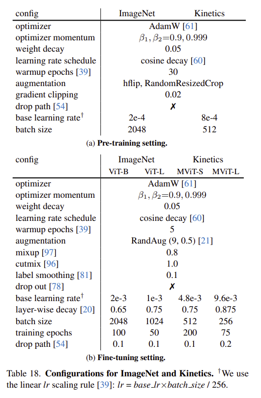
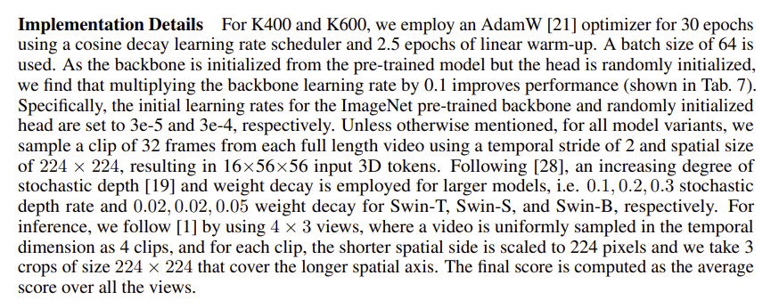
Optimizer setting

The optimizer and schedule used by the famous team should be good because their settings must be based on sufficient grid search. For example, I have been keep following the setting used by:

• Christoph Feichtenhofer and his team of the Facebook AI Research (FAIR). Their github repositories pytorchvideo and the SlowFast
• Wang liming of Multimedia Computing Group, Nanjing University. Their github repositories MCG-NJU

However, I don’t have much computational resource compared with the FAIR. Therefore, I also follows some settings that use fewer training epochs and smaller batch size.

Up-to-date collections (2022-05-07):

MaskFeat (slowfast)

• Cosine decay does NOT include restart, and it ends with 0.01 x base_lr
• Warmup starts from 0.01 x base_lr
• It seems that all runs in slowfast use max_norm=1.0 for clipping the grads, e.g. MViT has CLIP_GRAD_L2NORM: 1.0 in its config, which points to torch.nn.utils.clip_grad_norm_. However, the max_norm used by mmaction2 normally is 40/20.

VideoSwin:

My current pratice:

30 epochs:

# optimizer
optimizer = dict(type='AdamW', lr=3e-4, weight_decay=0.01)  # decay=0.05 if very large backbone
# optimizer = dict(type='AdamW', lr=3e-4, paramwise_cfg=dict(custom_keys={'backbone': dict(lr_mult=0.1)})) # if pretrained backbone
optimizer_config = dict(grad_clip=dict(max_norm=40)) # max_norm=1.0 if very large backbone
# learning policy
lr_config = dict(policy='CosineAnnealing',
                 min_lr_ratio=0.01,
                 warmup='linear',
                 warmup_ratio=0.01,
                 warmup_iters=2.5,
                 warmup_by_epoch=True)
total_epochs = 30

data = dict(
    videos_per_gpu=32, # batch size=32x2=64, where 2 is the number of gpus 
    ...

50 epochs:

# optimizer
optimizer = dict(
    type='SGD',
    lr=1e-3,
    momentum=0.9,
    weight_decay=0.0001)
optimizer_config = dict(grad_clip=dict(max_norm=40, norm_type=2))
# learning policy
lr_config = dict(policy='step', step=[20, 40]) # or [10, 20] for 25 poech 
total_epochs = 50

200 epochs

# optimizer
optimizer = dict(type='AdamW', lr=1e-4, weight_decay=0.05)
optimizer_config = dict(grad_clip=dict(max_norm=1.0))
# learning policy
lr_config = dict(policy='CosineAnnealing',
                 min_lr_ratio=0.01,
                 warmup='linear',
                 warmup_ratio=0.01,
                 warmup_iters=20,
                 warmup_by_epoch=True)
total_epochs = 200

data = dict(
    videos_per_gpu=16, # batch size 16 * 2 = 32, where 2 is the number of gpus 
    ...

Tips:

• There is a known linear scaling rule – When the minibatch size is multiplied by k, multiply the learning rate by k.
• Warmup seems to be impactful when the backbone network is Transformer (ActionFormer, Liyuan Liu 2020).

Loss quantization

Cross Entropy

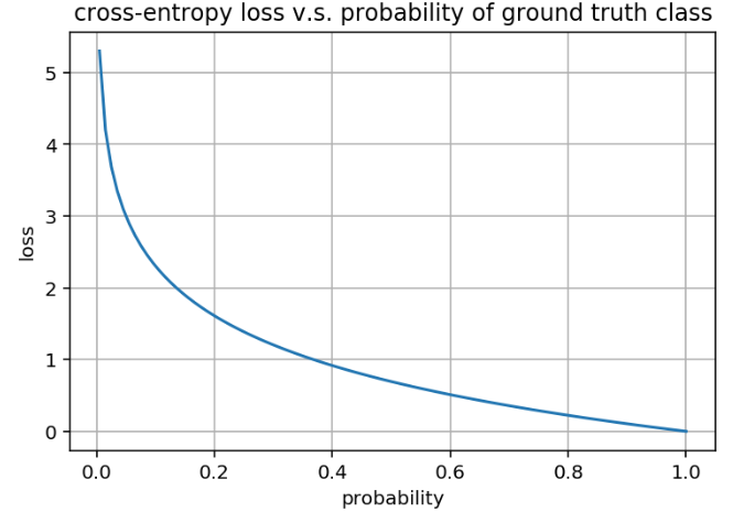
Prob. of GT	Loss	Comment
0	100
0.01	4.61	:disappointed: exploding gradient?
0.1	2.30
0.2	1.61
0.3	1.20
0.4	0.92
0.5	0.69	:neutral_face: meaningful
0.6	0.51	:flushed: it works
0.7	0.36	:grinning: good
0.8	0.22	:wink: great
0.9	0.11	:relaxed: pretty good
0.95	0.05
0.99	0.01	:triumph: perfect

GIoU

Copied from https://giou.stanford.edu/:

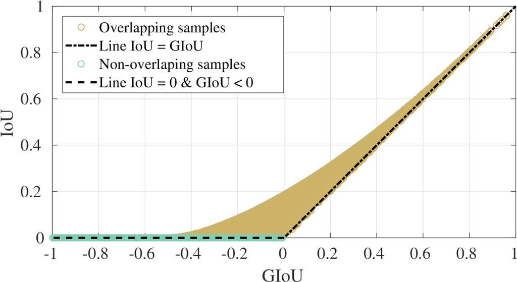
• Note that GIoU and IoU do not one-to-one map to each other. For example, the bbox-paris with different GIoU may have the same IoU, vice versa.
• The brown area are pair-samples overlapping with each other.
• Normally the GIoU is close to the IoU when the IoU is close to 1 or when the overlapping samples have similar x/y postion, otherwise the GIoU is smaller than the IoU.
• GIoU_loss equals 1 - GIoU

Miscellaneous

Position of Normalization Layers

[1] On Layer Normalization in the Transformer Architecture [2] A ConvNet for the 2020s [3] Understanding the Difficulty of Training Transformers [4] RealFormer: Transformer Likes Residual Attention [5] Blog [6] CogView: Mastering Text-to-Image Generation via Transformers

Let’s start with the Transformer. There are two kinds of known choices for the location of normalization: Post-LN and Pre-LN. Pre-LN is proposed newly than the Post-LN.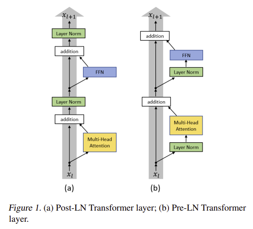

Conclusion:

• Post-LN is relied and sensitive to the Warm-Up[1]， because “the Post-LN Transformer cannot be trained with a large learning rate from scratch”[1].
• Pre-LN is NOT sensitive to the Warm-Up, and “Pre-LN Transformer converges faster than the Post-LN Transformer”[1].
• Post-LN is NOT as stable as Pre-LN, but it optimal performance is better[3][4][5].
• Pre-LN is recommended for easy training, while Post-LN is recommended when high performance is the target, at the cost of manul engineering, e.g. the Admin initilization [3] and the Warm-up.

What about CNN? Below is the block structure of the latest ConvNext:

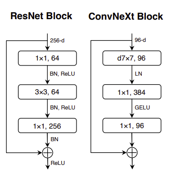
Conclusion:

• The widely used Batch-Normalization layers are now replaced by the Layer-Normalization layers. BTW, the amount is reduced.
• The Pre-LN is recommended.

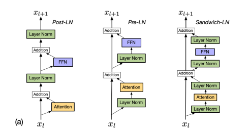
Extra: There is a technique called Sandwich-LN in transformer [6] to alleviate the value explosion problem:

Video backbone benchmark

	Source	top1	Params (M)	GFLOPs	Memory (M)	Training speed	Testing speed
I3D	github	71.1%	27.90	12.29	1721	18.7 iter/s	80.0 iter/s
I3D	mmaction2	73.3%	27.22	16.74	1751	16.5 iter/s	87.5 iter/s
SlowOnly	torchhub	75.6%	31.63	84.36	-	-	-
SlowOnly	mmaction2	75.6%	31.63	84.36	2987	4.9 iter/s	34.5 iter/s
X3D-M	torchhub	76.2%	2.01	5.07	-	-	-
X3D-M	mmaction2	75.6%	2.09	5.15	2257	9.8 iter/s	80.0 iter/s
MViT-B	torchhub	80.2%	36.30	70.8	3151	10.2 iter/s	35.3 iter/s

• top1 is reported on the kinetics400 validation set but are directly coied from the paper/repo. These work use different input resolution and training/testing data augmentation, thereby the top1 here is just for reference. It makes NO sense to consider together the top1 and the other variables. While generally speaking, the lower models are newer and should have higher best accuracy.
• Params and GFLOPs only calculate the backbone, while speed and memory involves the head.
• Input (N C T H W) is of shape (1, 3, 16, 224, 224).
• Params and GFLOPs are computed using the fvcore lib.
• Speed and memory evaluation are conducted on a single 2080ti GPU.
• Memory refers to the ocupied memory recorded by nvidia-smi during the training.

Mitigate negative transfer in sibling head

I encountered a problem that the classification head and the localization head in my model cannot come to their optima (val) at the same training phase. Specifically, the classification metric started to decline (overfitting) while the localization metric is still rising (underfitting).

I tried the below two methods for motigating this problem ref.

• Classication-aware regression loss (CARL)
• Guided loss

Video Data augmentation

Training augmentation

RandomResizeCrop and RandomRescale

There are two widely used training data augmentation on the spatial view of input video:

• Resize(-1, 256) - RandomResizedCrop(scale=(0.08, 1.0), ratio=(0.75, 1.33) - Resize(224, 224)
• RandomRescale(256, 320) - RandomCrop(224, 224)

		Resize(224)	Resize(-1,224)-Center(224)	Resize(-1,256)-Center(224)	Resize(-1,224)-Three(224)	Resize(-1,256)-Three(224)
ResizeCrop	Cls Acc	72.29	74.76	74.23	74.88	73.81
	Reg MAE	16.63	16.42	16.53	16.15	16.26
	Iter/s	477.3	525.0	479.8	183.7	156.1
	mAP@0.5	39.4%	42.8%	43.3%	42.7%	41.7%
RescaleCrop	Cls Acc	70.96	74.50	74.48	74.78	74.76
	Reg MAE	16.85	16.29	16.40	16.01	16.01
	Iter/s	495.8	514.6	502.4	178.8	161.8
	mAP@0.5	36.4%	41.9%	42.7%	41.6%	41.3%

Mixup

Mixing up two samples for data augmentation: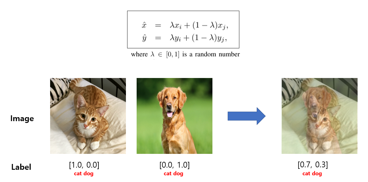

A psudo code:

beta = Beta(alpha, alpha)
lambda = beta.sample()
rand_index = torch.randperm(batch_size)
mixed_images = lambda* imgs + (1 - lambda) * imgs[rand_index, :]

The pdf of lambda under different alpha for mixup: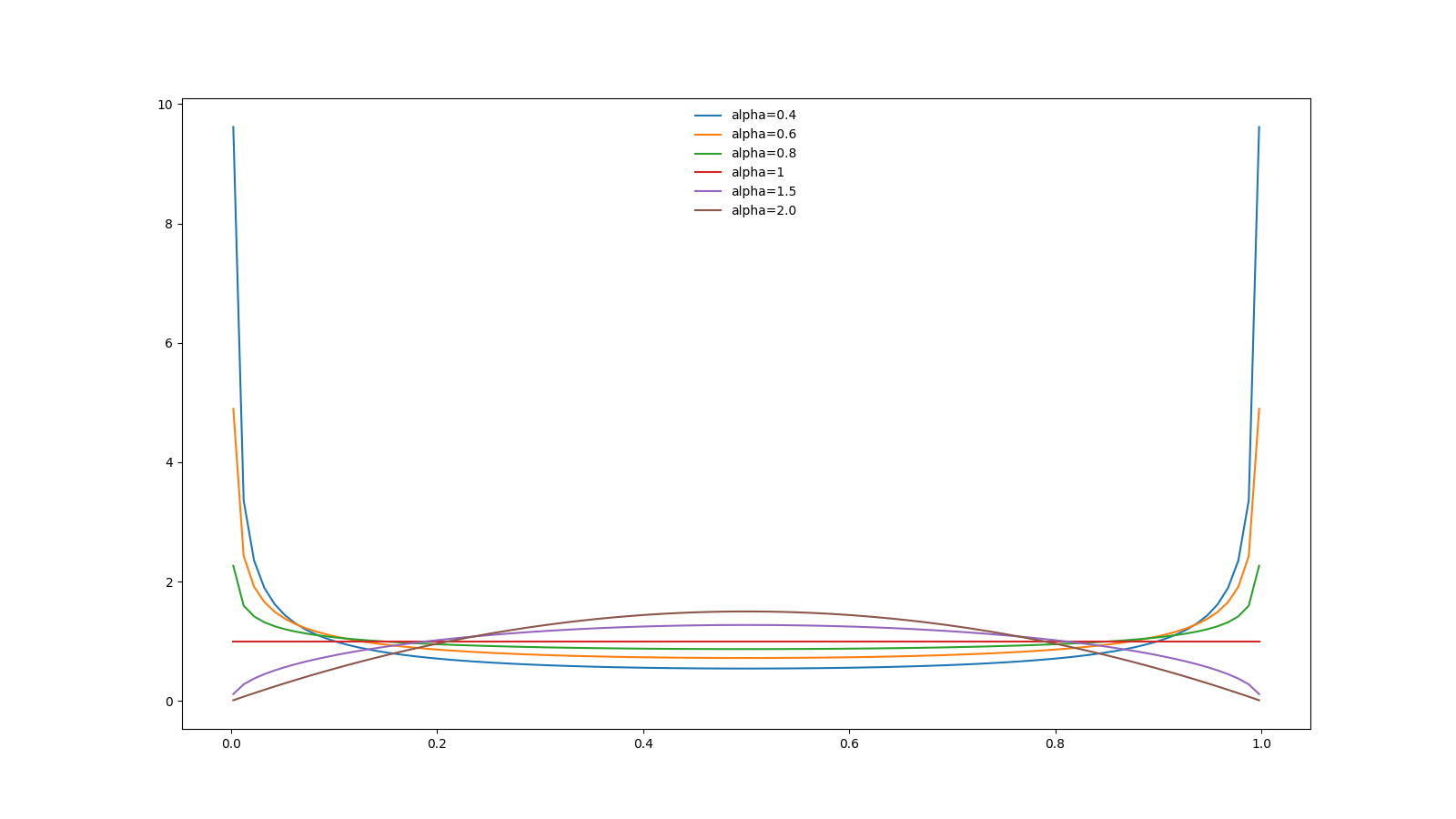

• From the above figure, we can conclude that a small alpha tends to sample values closing to 0 or 1, which represent a weak mixup.
• The strongest mixup is when lambda = 0.5. As the alpha increases, the probability intensity of lambda abound 0.5 is increasing.
• In short, largger alpha, stronger mixup.
• alpha=1 represents uniform distribution.
• alpha=0.8 is adopted in the MViT for training action recognition on Kinetics400.

Cutmix

Cutting subregions from two samples and mixup them for data augmentation:

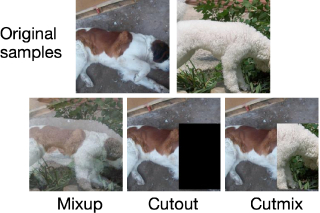
Similar to the mixup, because the strongest cutmix is when the lambda=0.5, larger alpha represetns stronger cutmix. FYI, alpha=1.0 is adopted in the MViT for training action recognition on Kinetics400.

One may argue that the lambda=1.0 should be the strongest mixup/cutmix. While because the label will also be mixed, so when lambda=1, the two samples are just simply exchanged after the mixup/cutmix.

Visulizing Beta distribution online

Essay

• Kinetics 400 (trimmed) occupies 10Mb for each video of RGB rawframes. 30Mb for each video of (optical flow+ RGB) rawframes.
• ActivityNet200 (untrimmed) occupies 3.3Gb for each video of RGB rawframes. 10Gb for each video of (optical flow+ RGB) rawframes.
• GMA optical flows of the validation set (19404 videos) of Kinetics 400 occupy 61G disk size, showing that each video occupies about 3.21Mb. So training set of 240618 videos should occupies about 800G.
• Training on remote server but want to auto-save the produced files in local machine? Check [here]
• Convolution perforsm parameter-dependent scaling and content-independent interaction. While self-attention is the opposite. About point 1, for the CNN, the number of parameters depends on the size of the receptive filed (7x7 kernel has more parameters than 5x5), while for the self-attention, the number of parameter is independent with the “receptive filed”: the number of parameter is the same no matter using local-self-attention or global-self-attention. About the point 2, for the CNN, the interaction between the pixel/feature is independent with the content of pixel/feature: the kernel values is shared at different position. While the interaction beween the patch/feature in self-attention depends on the content of the patch/feature: the attention (interaction) is computed based on the token values.
• The typical format of bounding boxes in object detection is (x1, y1, x2, y2) where (x1, y1) and (x2, y2) are the coordinates of left-top and right-bottom points of bboxes, respectively. Note that the left-top pixel of image is the origin, i.e., (0, 0). See ref1 and ref2.